Disclaimer: This post is based on an exercise session on $k$-means for the course Mathematics of Signals, Networks, and Learning (2024) at ETH Zurich. These exercise sessions focus on further topics, while the main course material is covered in lectures. See also the excellent lecture notes by A. S. Bandeira and A. Maillard. Some of the statements in this post are left as exercises because they appear in homework or during exercise sessions.
Warm-up and Introduction

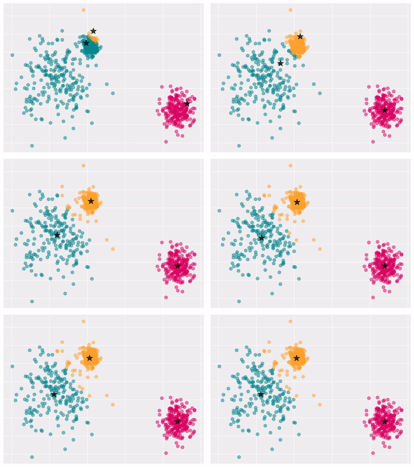
Figure 1 Convergence of k-means algorithm
Let us briefly recall perhaps one of the simplest methods for clustering, $k$-means clustering.
Given $x_1, \dots, x_n \in \mathbb R^p$, the $k$-means clustering partitions the points into clusters $S_1, \dots, S_k$ with centers $\mu_1, \dots, \mu_k\in \mathbb R^p$ as the solution to: \begin{equation}\label{eq:kmeans} \min_{\substack{S_1, \dots, S_k\\ \mu_1, \dots, \mu_k}} \sum_{\ell=1}^k \sum_{i \in S_\ell} \|x_i - \mu_\ell \|^2. \end{equation}
Unfortunately, this problem is not easy to solve with efficient methods: indeed, it is proven to be NP-hard (which means that assuming $P \ne NP$ there is no polynomial time algorithm solving the worst-case instance).
Observe that if we know the cluster centers it becomes easy to find the corresponding partition that minimizes objective. Vice versa, it is easy to compute cluster centers when partitions are known. This observation lies at the core of the Lloyd’s algorithm.
Lloyd’s algorithm outputs a (local) optima of \eqref{eq:kmeans}. It iteratively updates the clusters $S_1, \dots, S_k$ and the centers $\mu_1, \dots, \mu_k$ as following:
-
Given a choice for the partition $S_1 \cup \cdots \cup S_k$, the centers that minimize \eqref{eq:kmeans} are given by \(\mu_\ell=\frac{1}{\left|S_\ell\right|} \sum_{i \in S_\ell} x_i .\)
-
Given the centers $\mu_1, \ldots, \mu_k \in \mathbb{R}^p$, the partition that minimizes \eqref{eq:kmeans} assigns each point $x_i$ to the closest center $\mu_k$.
Lloyd’s algorithm always converges; though, not always to a global optimum.
Cluster convexity
Clusters from the above procedure can also be defined as regions in $\mathbb R^p$, rather than a subset of data points. In this case, clusters $S_\ell \subseteq \mathbb R^p$ are such that $S_1 \cup \cdots \cup S_k = \mathbb R^p$ and $\ell$-th cluster $S_\ell$ consists of points that are closer to $\mu_\ell$ than to other cluster centers. One of the properties of the clusters defined in this way is that they are convex.
We proved this proposition in class. For readers who were not present or who want to recall the proof, I invite you to prove it yourself. Here is a hint:
Recall the definition of a convex set.
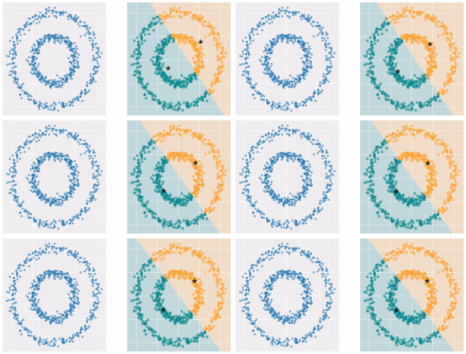
A direct implication of this property is the fact that $k$-means may not lead to a good clustering when clusters are not convex, see Figure 2 for such an example.

Figure 2 Lloyd’s algorithm convergence on data with non-convex clusters. The left plot shows the original data, and the right plot illustrates iterations of Lloyd’s algorithm applied to the data. $k$-means struggles to capture the cluster structure, because the original clusters are non-convex.
Remark. The above figure provides another hint for the proof of Proposition 1. Consider the decision boundary between any two clusters produced by Lloyd’s algorithm. What does this boundary look like? What can you say about boundary of any decision region? Can you see a connection to the Voronoi diagram?
Additionally, in which situations can Lloyd’s algorithm also successfully cluster data with non-convex clusters?
Initialization and $k$-means++
Lloyd’s algorithm, described in Introduction, lacks a crucial ingredient — initialization. The quality of the algorithm’s output significantly depends on the initial cluster centers chosen.
A very simple, though not very effective, strategy to select initial centers is to choose them randomly from the input points. A quick simulation shows that this approach often fails even on simple instances of three well-separated convex clusters (see Figure 3). Furthermore, different runs of Lloyd’s algorithm with random initialization can lead to drastically different clustering results, making the initialization approach very unstable.
Figure 3. Lloyd’s algorithm is sensitive to initialization. The left plot illustrates the clustering quality for 100 different random seeds, measured by the Rand index (a measure of similarity between the resulting data clustering and the true underlying clusters). The right plot shows the suboptimal convergence results of the clustering for one of the random seeds.
One reason for suboptimal algorithm convergence is when two initial centers fall in the same cluster. To avoid this issue, one may devise another strategy: choose the first cluster at random and then select all subsequent cluster centers as the furthest points from the previously chosen centers. However, this greedy approach can again lead to algorithm sensitivity issues. More specifically, if the data contains a few outliers, these outliers may be selected as initial cluster centers, significantly distorting the clustering results and leading to poor overall performance of the algorithm.
To combine the best of both worlds, we utilize probabilistic techniques. We choose cluster centers iteratively, with the next center chosen randomly from the data points with a probability proportional to their shortest distance from the chosen centers. If there is a natural cluster of points, it is likely that the next center will be chosen from that cluster. On the other hand, this algorithm is less sensitive to outliers if there are only a few. This idea lies at the core of the $k$-means++ procedure for initialization. The procedure is listed in the display below.
    \begin{algorithm}
    \caption{$k$-means++}
    \begin{algorithmic}
    \INPUT  Dataset $X = \{x_1, x_2, \ldots, x_n\}$, Number of clusters $k$
    \OUTPUT Initial set of centers $C = \{\mu_1, \mu_2, \ldots, \mu_k\}$
    \STATE Choose one center uniformly at random from among the data points, $\mu_1 = x_j$, where $j \sim \mathrm{Unif}([n])$
    \FOR{$i = 2$ \TO $k$}
        \STATE For each data point $x$ compute the distance to the nearest center
        $d(x) = \min\limits_{j = 1, \dots, i} \|x - \mu_j\|$
        \STATE Choose $x_j$ at random as a new center with probability $\mathrm{Prob} ( \mu_i = x_j ) = \frac{d(x_j)^2}{\sum_{\ell=1}^k d(x_\ell)^2}.$
        \STATE $C \gets C \cup \{\mu_i\}$
    \ENDFOR
    \end{algorithmic}
    \end{algorithm}
Remark Combining exploration (choosing points uniformly at random) and exploitation (choosing the furthest point) is a popular technique in randomized algorithms. It often improves algorithm performance compared to using these approaches individually. See also the discussion in the last section, Conclusion and further connections.
This initialization is often used in practice for Lloyd’s algorithm. In the popular Python library scikit-learn, $k$-means++ is used as the default initialization for the implementation of Lloyd’s algorithm in KMeans().
Eventhough, this procedure is quite effective already after one run, in modern applications (including the mentioned scikit-learn’s implementation of $k$-means), the algorithm is run several times for higher stability.
While this initialization does improve performance, there are still situations where Lloyd’s algorithm converges to a local optimum. These scenarios include clusters of very different sizes, clusters with different variances, and anisotropic clusters (i.e., not ‘spherical’, or mathematically, not isotropic). For more details, see this scikit-learn demo. Figure 4 duplicates the one from the mentioned demo and summarizes the main limitations of $k$-means.
Figure 4. Performance of Lloyd’s algorithm on 4 different scenarios: choosing wrong number of clusters, anisotropic clusters, clusters of different variances, and clusters of different size.
Let us briefly discuss some potential fixes. To determine the number of clusters, one can use average silhouette method or elbow method. For non-convex or anisotropic clusters, the data can be pre-transformed so that the new data satisfy the assumptions of $k$-means. The combination of applying the pre-transformation and $k$-means can also be seen as the kernel $k$-means. However, in some settings, it is a priori not clear which transformation should be chosen, especially when the data is high-dimensional. In these situations, using other clustering techniques may be more beneficial. We explore some of the alternative methods in the next section.
Other clustering algorithms
A method related to $k$-means is the Gaussian Mixture model (GMM, in short). The model assumes that data follows a Gaussian mixture (i.e., each cluster follows a Gaussian distribution). This model can overcome some of the issues mentioned in the previous section, such as anisotropic clusters, different variances, and an unequal number of samples in each cluster. However, this method is still ill-suited for non-convex clusters due to its assumptions.
Remark (for those of you acquainted with the EM algorithm): The EM algorithm for finding clusters in GMM can be seen as a probabilistic version of Lloyd’s algorithm. Indeed, the maximization step is similar to calculating the new centers, and the expectation step is similar to assigning points to clusters. Note that the expectation step provides scores instead of hard assignments. This is often called soft clustering. This means that the model provides a probability vector of uncertainties. For example, if we have three clusters and the resulting score vector for a point is $(0.7, 0.23, 0.07)$, it means that the model has a 70% certainty to assign this point to the first cluster, 23% to the second one, and 7% to the third one. We can choose the resulting clusters by taking the cluster with the largest probability.
There exist many other clustering algorithms. Popular methods with good performance include spectral clustering, DBSCAN, and HDBSCAN. We will not discuss them in detail, but an interested reader is welcome to compare these methods in the Overview of clustering methods on scikit-learn website.
Conclusion and further connections
$k$-means is an intuitive and very simple clustering method. Besides introducing the method itself and its strengths and limitations, we demonstrated two important mathematical techniques on this method.
First, recall that the original objective function is, in general, NP-hard. To make this problem tractable, we used an iterative procedure to successively approximate a (local) optimum. A prominent example of an iterative procedure is the gradient descent method for finding an optimal solution to a differentiable function. Another example is the fixed point iteration.
There is more to it than just iterative estimation of the solution. Recall that Lloyd’s algorithm is a two-step procedure where we iteratively optimize part of the parameters while keeping others fixed, and then optimize the latter parameters while keeping the former ones fixed. The same idea lies in the expectation-maximization (EM) algorithm for Gaussian mixture models and, more generally, for finding maximum a posteriori estimates of parameters in statistical models with latent (hidden) variables. You can encounter a similar technique in the alternating projection method for finding a point in the intersection of two convex sets, where one alternates from a projection onto one set to a projection onto the other set. There are many more examples of this technique; can you recall any other use cases?
The second technique we encountered is combining exploration and exploitation to improve algorithm performance. A few other more advanced examples are the randomized Kaczmarz algorithm for finding a solution to an overdetermined linear system, and randomized matrix multiplication. You can learn more about these randomized algorithms in the monograph Randomized matrix computations: themes and variations.
You can find simulations for $k$-means (and other simulations related to other topics in the course) in this github repo.